- ABOUT
- PRODUCT
-
CASES
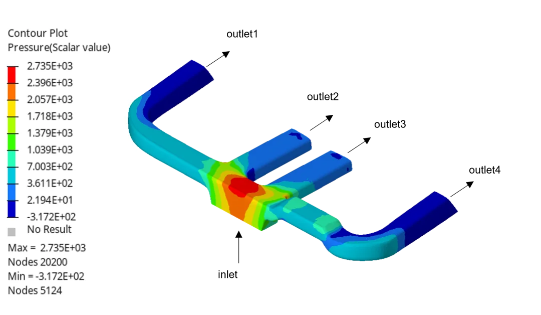
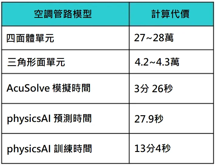
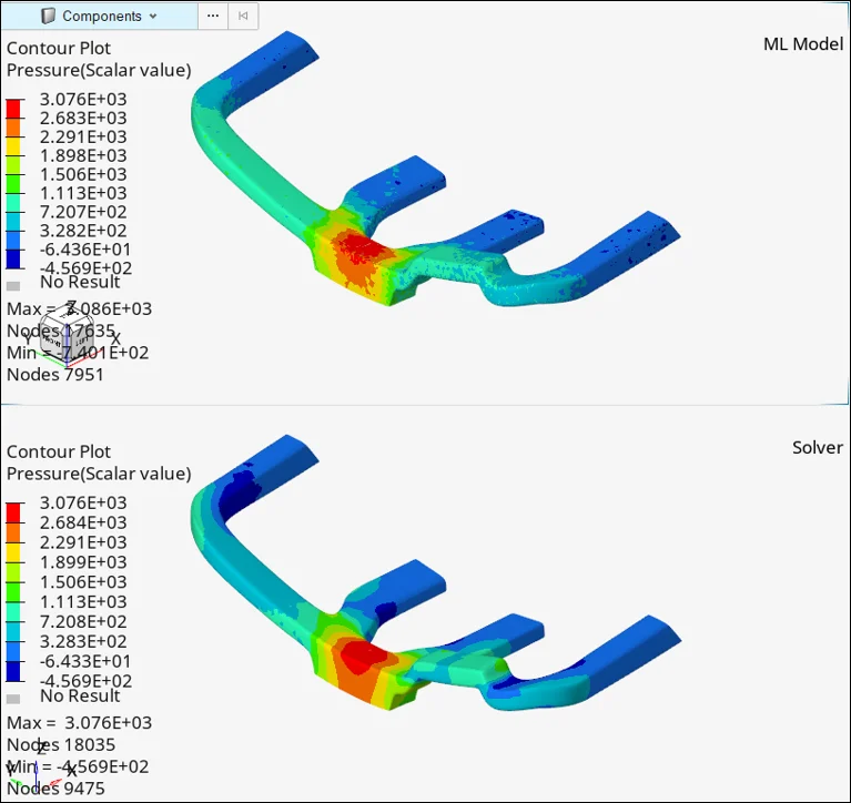
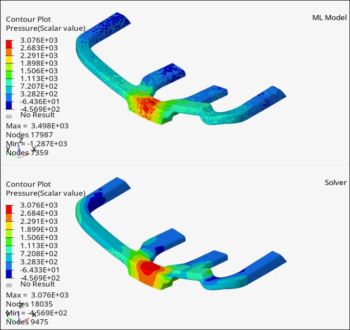
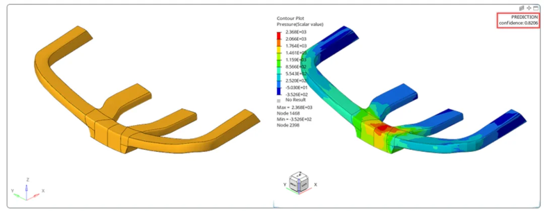
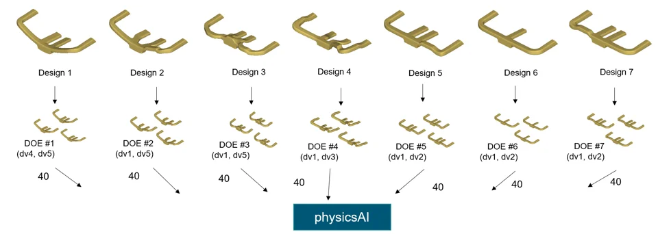
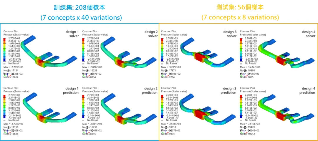
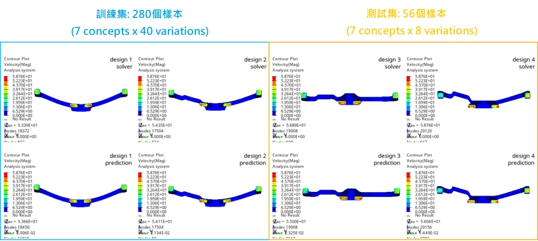
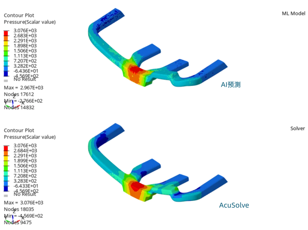
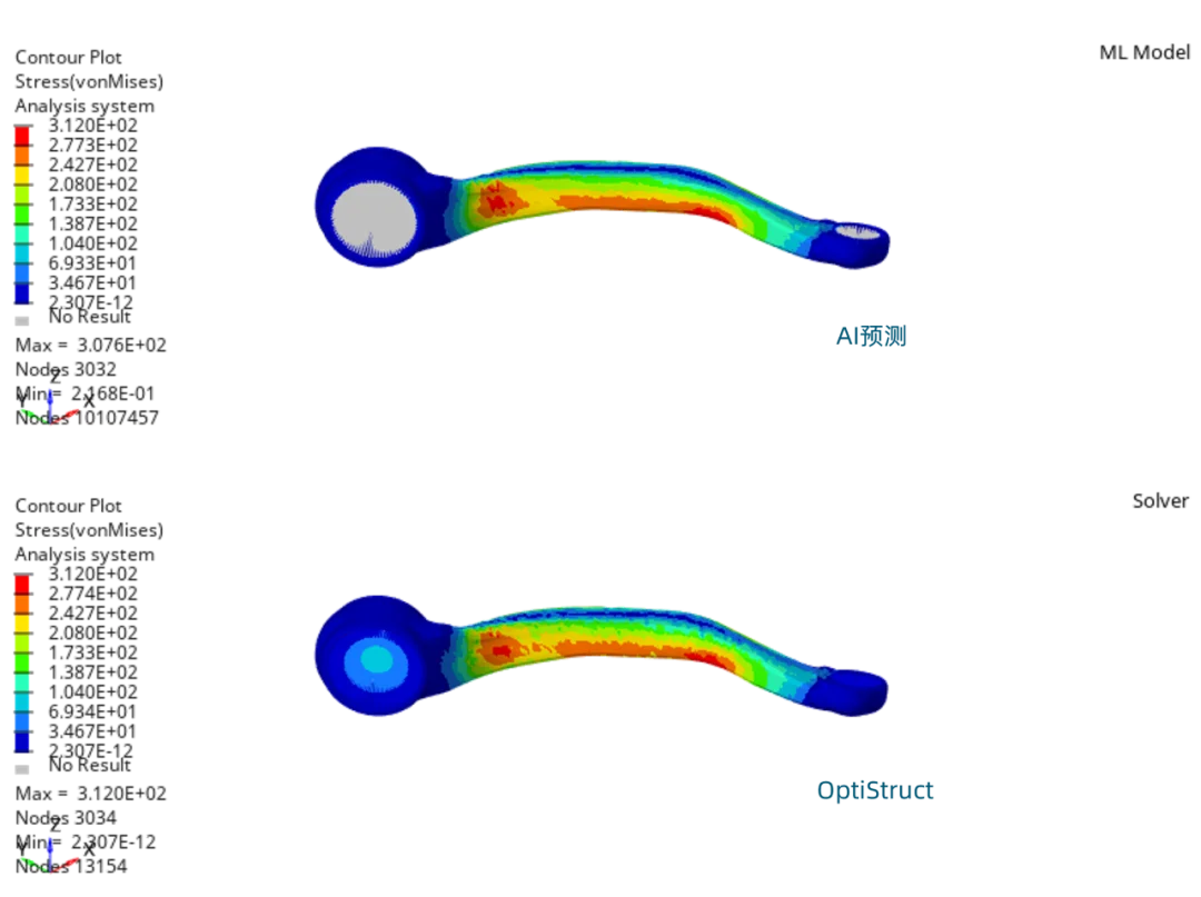
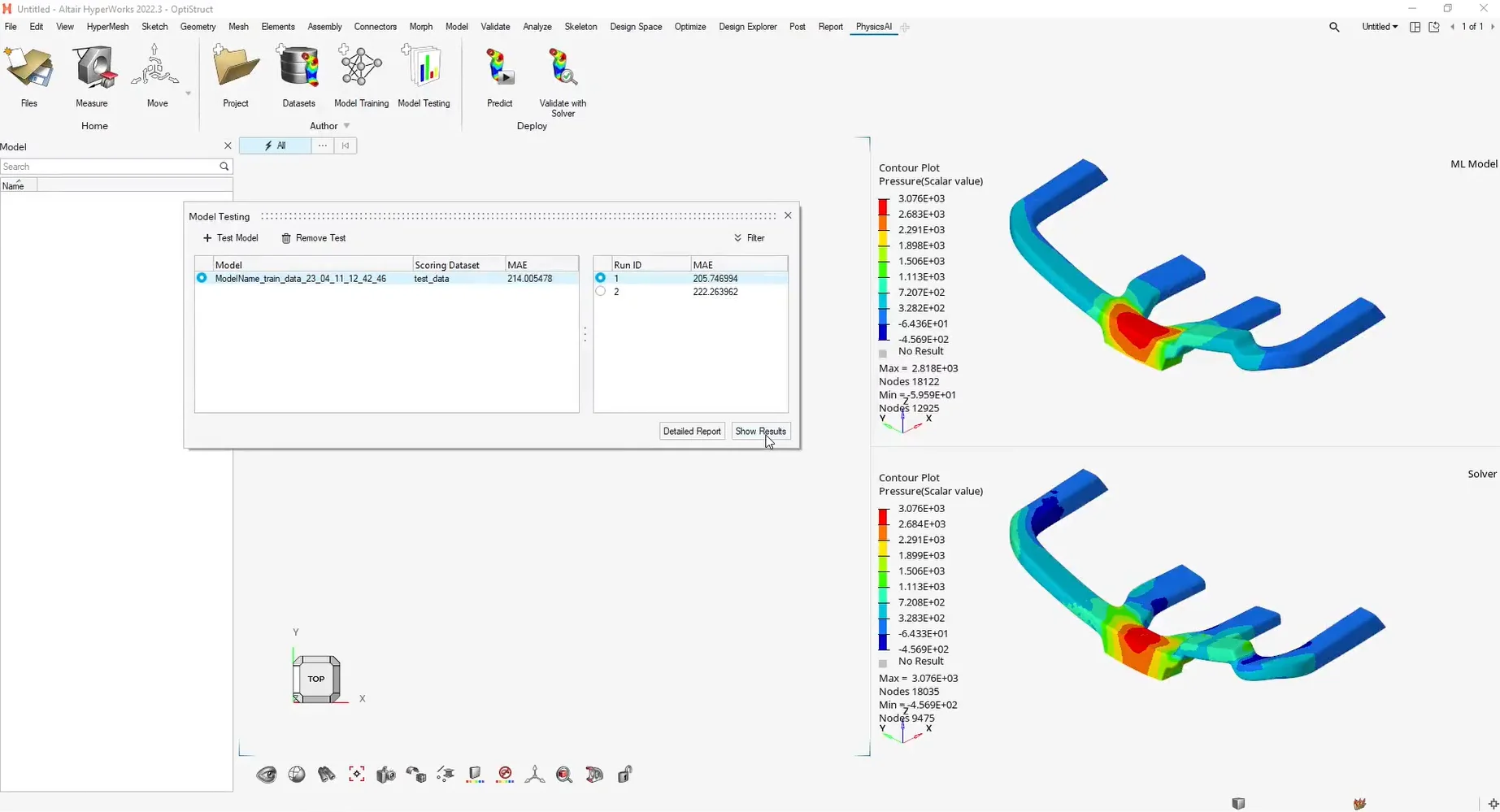
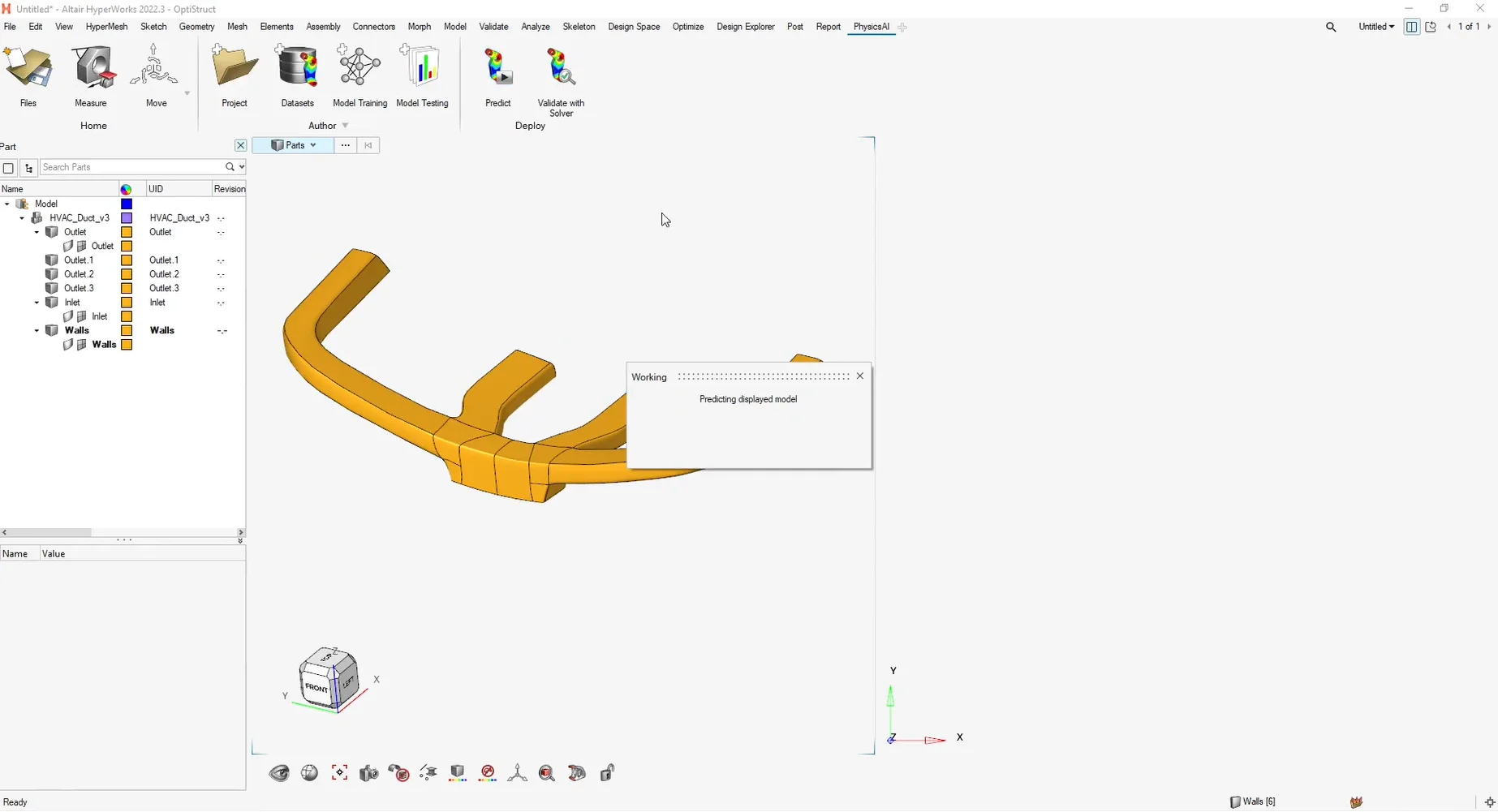
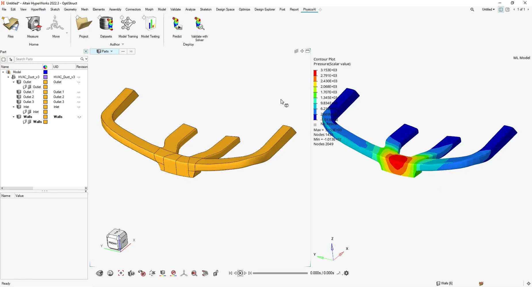
AI|Mechanism ElectricPredicting the Structural Strength of Heavy-Duty Lifting Hooks with PhysicsAI Big Data Analysis of Air-Conditioning Performance Using AI Optimizing Cement Formulation with AI | RapidMiner AI Image Classification for Metal Processing Defects|RapidMiner Accurately Predicting Spring-Clip Stress Using AI Data Analytics|physicsAI Optimizing PCB Fastening-Point Locations Using AI Data Analytics|ExpertAI Motor Performance Prediction Using AI Data Analytics|Knowledge Studio Bearing Failure Prediction Using AI Data Analytics|RapidMiner Robotic Arm Failure Prediction Using AI Data Analytics|RapidMinerAI|Vehicle AeroPredicting EV Liquid-Cooling Radiator Performance with physicsAI Using AI to Predict Wheel Stress AI-Based Detection & Localization of Metal Processing Defects | RapidMiner Multidimensional Frame Optimization Using AI Data Analytics|ExpertAI Predicting Vehicle Frame Structural Stress Using AI Big Data Models|Knowledge Studio Predicting Bicycle Fork CAE Results Using AI Data Analytics Models|physicsAI CFD Flow-Field Prediction for Automotive Air-Conditioning Piping|physicsAICAE|ElectronicElectromagnetic Field Analysis of Wireless Power Transmission Devices | Flux Electromagnetic Field Analysis of High-Power Transformers | Flux Packaging Drop-Test CAE Analysis and Topology-Optimized Design |Radioss PCB Modeling and Thermo-Mechanical Coupling Analysis Case Study|SimLab x OptiStruct Server Drop-Test Analysis – Enhanced with Richin Technology’s Customized HyperMesh Scripting|HyperMesh x Radioss x HyperStudy Rapid Keyboard Assembly & Drop-Test CAE Analysis|SimLab x Radioss Fast Modeling Techniques for Electronic Products|HyperMesh Completing Complex Mouse CAE Modeling at 10× Speed|SimLab Drop & Impact Analysis for Electronic Products | Radioss Read More...CAE|MechanismCFD Thermal Performance Analysis of Transformers Magnetic Component Design & Analysis for High-Voltage, High-Power Converters Sewing Machine Electro-Control System Simulation|Embed Integrated Analysis of Motor and Drive Control|FluxMotor x Flux Motor Design Analysis for Electric-Assist Bicycles|FluxMotor Multidisciplinary Motor Optimization Design|Flux Motors Application of EDEM in Hammer Crushing Pneumatic Nail Gun Firing Analysis | Fluid–Structure Interaction (FSI) Gearbox Lubricating-Oil Cooling CAE Analysis|nanoFluidX Read More...CAE|Vehicle AeroGap Analysis and Optimization of Rocket Fairing Locking Mechanisms Multiphysics CAE Analysis of Battery Packs Bus Rollover Impact Analysis(ECE R66) Wheel Rim Optimization Analysis Vibration and Fatigue Durability of Motorcycle Frames Automotive Vibration and Fatigue Durability Landing Gear Retraction, Deployment & Control Analysis Fluid–Structure Interaction (FSI) Analysis of Composite UAVs UAV Flow-Field Load Input Analysis – True-Load Loads Read More...CAE|ConstructionOptimizing Exhaust & Fresh-Air Duct Ventilation in Underground Parking Facilities Using CFD Selecting Vegetation Using Building CFD Wind-Field Simulation Analysis|AcuSolve Structural Strength Analysis of Large Automated Storage Systems|SimSolid Water Droplet Analysis in an Exhaust Gas Scrubber|AcuSolve x EDEM Building CFD Wind-Field Analysis|AcuSolve Structural Strength Analysis of MRT Platform Screen Doors|HyperWorks Structural Strength Analysis of Outdoor Art Installations|HyperWorks Fluid–Structure Interaction (FSI) Analysis of a Metal Flower Sculpture
-
TECHNOLOGY
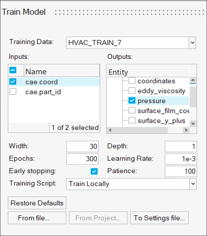
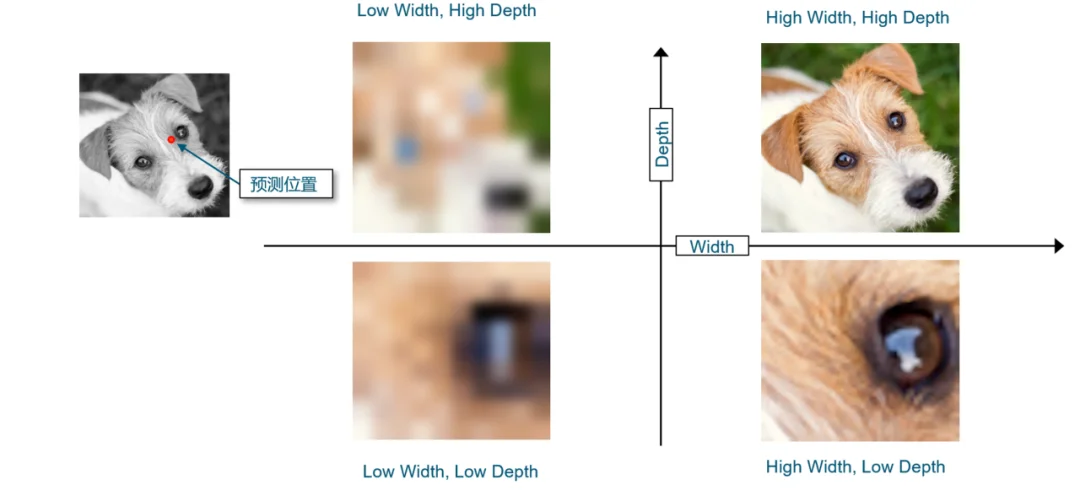
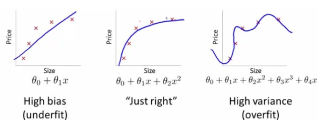
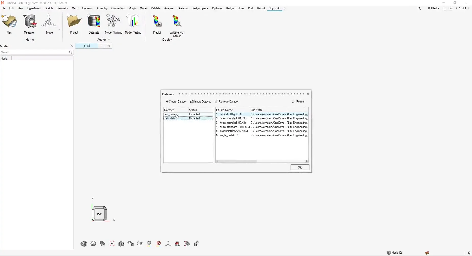
HyperWorks NewVersionAltair 2023 HyperWorks New Release Launch Event HyperWorks Latest Version / All Versions【Hardware Requirements】 【HyperWorks 2025.1 】New Releases – Article Overview 【Inspire Motion 2025.1】Major Leap in New Features Unveiling the New Pre-Processing Highlights in【HyperMesh 2025】and【SimLab 2025】 【Altair PhysicsAI 2025 】Key New Features 【OptiStruct 2025~2025.1】New Technical Highlights HyperWorks 2025 New Features Overview and the Future Outlook for PhysicsAI Applications HyperWorks 2025.1 New Release
(Installer Download & Hardware Requirements) Read More... - NEWS
- CONTACT